Scalable silhouette estimation

Here I am, writing my first official blog! And surprise surprise, it is about a recent work we published as a preprint on arXiv.

The title of our work is Scalable and Distributed Silhouette Approximation, with my amazing coauthors F. Altieri, A. Pietracaprina, G. Pucci and F. Vandin.

What is it about?

In data-analysis we often need to cluster a dataset by optimizing an objective function, popular objectives are \(K\)-means, \(K\)-center, spectral clustering on graphs or anything you prefer.

But here it comes the issue, consider the following three situations:

1. You do not know how many \(k\)-clusters your dataset is supposed to contain;
   1. You try different values of \(k\) if your algorithm allows you to set such parameter;
   2. You are given \(k\) clusters in output and your algorithm claims this is the best it can do;
2. You know your dataset has exactly \(k\) clusters, however you are running different algorithms (with different parameters and possibly different objectives). Which solution should you trust?

It seems a complete nightmare! Luckily here it comes your solution: the silhouette coefficient.

Silhouette definition

The silhouette¹ rescues all above issues as follows.

Say that you obtained your clustering \(\mathcal{C} = \{C_1,\dots, C_k\}\) of your dataset \(X = \{ e_1,\dots,e_n \}\) lying in some metric space \((X,d)\). The silhouette is a validation metric, providing a score \(s(e_i) \in [-1,1]\) for each element \(e_i\) of your dataset where

• \(s(e_i) \approx -1\) the element is badly clustered
• \(s(e_i) \approx 1\) the element is well clustered

Where for an element \(e_i\)

• badly clustered \(\to\) closer, on average, to the elements of my closest cluster than those of my cluster
• well clustered \(\to\) closer, on average, to the elements of my cluster than those of the closest cluster

Fixing \(e_i\) and its cluster \(C\) formally we have that the local silhouette is defined as

and

where \(s(e_i) = 0\) if \(\lvert C\rvert = 1\).

As always looking at an image can be much more worth it than starring at the formulas.

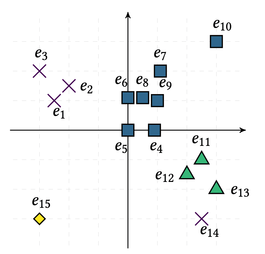
Consider the following clustered dataset (shapes tell us the clusters) on an Euclidean plane

Then under the Euclidean distance we can draw this nice silhouette plot 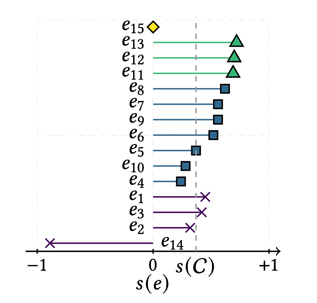The plot simply sorts all points per cluster according to the local values \(s(e_i)\) we can then do data analysis! As expected point \(e_{14}\) has a very bad silhouette, why?

Wait! What is \(s(\mathcal{C})\)? Well to score the global quality of \(\mathcal{C}\) we simply compute the average

Our contribution

I will start by briefly listing our key theoretical contributions.

For parameters \(\varepsilon, \delta\in(0,1)\) we get

• estimates \(\hat{s}(e_i)\) very close to \(s(e_i)\) as a function of \(\varepsilon\) and with error probability bounded by \(\delta\) we use: \(\mathcal{O}(n\varepsilon^{-2}\log(nk/\delta))\) total distance computations!
• an estimate of the global silhouette with similar accuracy and probabilistic guarantees using \(\mathcal{O}(n\log(nk/\delta) + mkt)\) distance computations where \(m\ll n\) and \(t\) depends on \(\varepsilon\) and \(\delta\).
• we show that all our algorithms can be ported in a distributed environment (e.g., the Massively Parallel Computing (MPC) model) using a constant number of rounds and sublinear local memory.
• it can be used for any metric distance, differently from many existing approaches.

That is it both local and global estimation methods use a subquadratic number of distance computations!

Why should I care, does it even compile?

• we show that we can process large datasets with millions of points extremely efficiently (i.e., less than 10 minutes)
• we provide an accompanying python package: that you can simply install with pip install silhouette-scalable

If you want to know more about the techniques underlying our contributions continue to the next section, otherwise that is!

Extra about our estimator

If you are curious of how we achieve our estimates let us start to look at what we are trying to estimate. In this context I will focus on the estimation of all values of \(s(e_i)\). So more formally the problem we are trying to solve is to obtain estimates \(\hat{s}(e_i)\) such that for given \(\varepsilon, \delta\in(0,1)\)

i.e., the usual \((\varepsilon, \delta)\)-approximation guarantees, where \(f(\varepsilon) = \frac{4\varepsilon}{1-\varepsilon}\), which for small \(\varepsilon\) is essentially linear (\(\approx 4\varepsilon\)).

By definition we know that: \(s(e_i) = \frac{b(e_i) - a(e_i)}{\max(b(e_i), a(e_i))}\) by looking at this formula your brain (mine for sure), will scream, just sample points!

Yielding our first approach:

1. sample a sublinear number of points from \(S\subseteq X\) (say each point of \(X\) is included in your sample with probability \(p\in(0,1)\))
2. evaluate \(\hat{s}(e_i)\) over the sampled points in \(S\), in particular estimating the values of \(a(\cdot)\) and \(b(\cdot)\) only using \(S\).

As always, with sampling algorithms the core is understanding how small \(S\) can be to obtain that our estimates are close within \(f(\varepsilon)\) from our actual values.

Here it comes the issue! It is a nice exercise to build an instance where no \(S\) obtained through uniform sampling and with size sublinear in \(n\) can escape a constant error, i.e., the error can never become arbitrarily small 🤯.

Hint: Think of the impact that single outliers can have on the terms \(a(\cdot)\) and \(b(\cdot)\) (or check our paper).

How we solve the issue. To address this problem we rely on a technique² that computes a weighted sample for each cluster \(C_j, j\in[k]\) which guarantees that for any query point \(e\) of the metric space the sampled points in \(C_j\) provide an accurate estimation of the sum \(\sum_{e'\in C_j}d(e,e')\). The intuition behind this approach is that it performs, two sampling phases per cluster \(C_j\). The first phase is used to identify points \(e'\in C_j\) that have high impact for terms \(\sum_{e'\in C_j}d(e,e')\) (i.e., they are somehow outliers with respect to the majority of elements in \(C_j\)). The second step obtains the weighted sample accounting for the computation in the first phase.

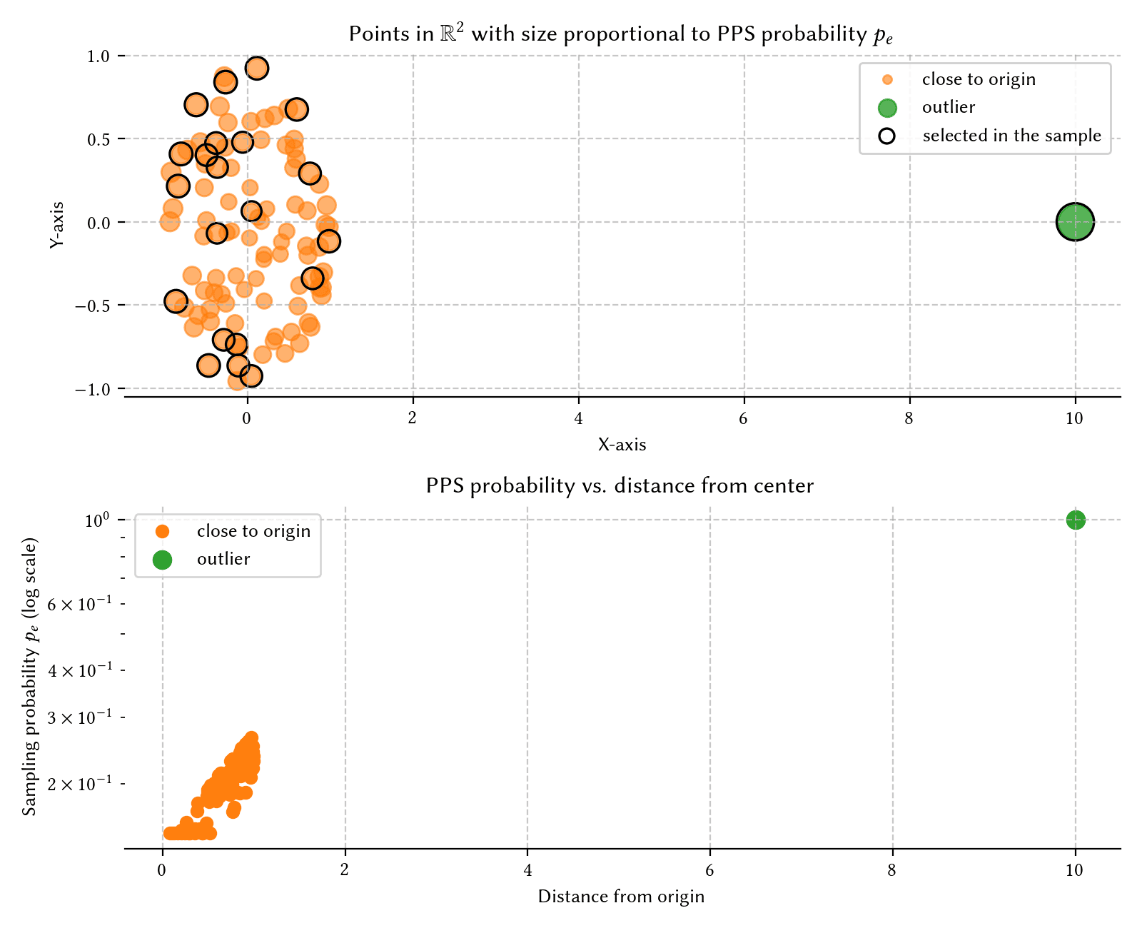
To provide you more intuition I generated a toy example where

• the top plot shows the geometry of the dataset, and there is a mark (black circle) over the sample collected with the computed probabilities by the PPS technique
• the bottom plot shows the distribution of the sampling probabilities of the points as a function of their distance from the origin

Loading from GitHub…

In our method, we use this weighted sample (with weights from PPS) to compute (probabilistic) estimates \(\hat{s}(e_i)\) with bounded error as desired (controlled by \(f(\varepsilon)\)), for all elements of \(X\).

For the global silhouette we use some other nice properties, but this post is already becoming too long, so I will cut it here!

On further reading

Since I particularly enjoy sampling techniques I highly recommend reading ² as it can be extremely helpful in many applications. (There also many interesting followup works and other applications!)

On the data analysis side, knowing about validation measures is also very important (especially if you are a practitioner), thus I suggest this nice survey³.

Acknowledgements

Thanks to Matteo Ceccarello for verifying that our library is up and running.

References